With the introduction of Time Series (or processes) in Analytic Solver V2020 (version 20.5.0.0), users can now represent their uncertain variables as a time series. Users of @RiskTM may be particularly interested in this new feature as Frontline has made it that much easier for models created in @Risk to be ran and solved in Analytic Solver.
In past versions of Analytic Solver, uncertain variables were represented by a distribution, which generated a single random number (scalar) at each trial. A Time Series is another type of uncertain variable, which generates a random numerical vector at each trial. As a result, a time series may be qualified as a generalized distribution to which a discrete time dimension has been added.
A Time Series is represented as a function in a formula containing optional property functions. Since a Time Series returns a numerical vector at each trial, the Time Series must be entered as an array. The size of the array formula determines the length of the Time Series.
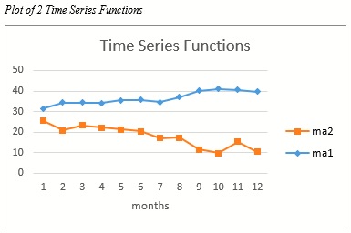
The discrete time dimension has the abstract values : {1, 2, 3, …, n} where n is the length of the series. The discrete units may represent the time in years, months, days, hours, etc. At each time point, the function generates a random number. As a result, a time series at a given trial can be drawn as a discrete curve with time values along the x-axis and random numbers along the y-axis.
Plot of 2 Time Series Functions

If 1000 trials are run in a simulation model, then there will be 1000 curves; one curve for each trial. Double clicking the cell containing the Time Series function will bring up a histogram showing all trials at a given time point.
A Time Series may be interpreted as an ordered set of joint distributions. If the joint distributions of a Time Series have the same mean and variance, the series is called stationary. If the joint distributions of a Time Series have the same mean but different variance, the series is called heteroskedastic.
Analytic Solver features 9 Time Series functions. Three optional Time series properties and three optional general properties may be applied to each function. See the Psi Property Functions section below.
Time Series Functions
Analytic Solver's Time Series functions are grouped into 2 categories
- Autoregressive Moving Averages (ARMA)
- Autoregressive Conditional Heteroskedasticity (ARCH)
Users should note the time series functions as implemented by Frontline Systems may contain some variation in the calculation when compared to @Risk's implementation. Users should check their models to ensure that the time series functions are behaving as expected.
Although Analytic Solver does not offer a fitting feature for a time series, Analytic Solver Data Mining does include fitting for ARIMA models. See the Analytic Solver Data Mining Reference Guide for more details.
See the two examples time series examples on the Simulation tab of Analytic Solver under Help – Example Models for an illustration of how a time series may be used in Analytic Solver.
Autoregressive Moving Averages (ARMA)
The ARMA time series (or processes), developed by Box and Jenkins in the 1970's, are well known and used extensively in practice. Theoretically, these functions are based on stationarity, meaning they have the same mean and variance, i.e. the time series is constant throughout time. If this assumption is not true, the time series data can be transformed using logarithms, differences and/or de-seasonalizing in order to induce stationarity. Afterwards, an ARMA process is applied to reversely transform the data using exponentiating, integration, and/or seasonalizing.
ARMA processes are, in general described by integer values p and q where p is the number of autoregressive terms and q is the number of moving average terms. Analytic Solver features five ARMA functions where p + q is less than or equal to 2: AR(1), AR(2), MA(1), MA(2) and ARMA(1,1).
Autoregressive Conditional Heteroskedasticity (ARCH)
The ARCH time series functions were developed in more recent times in order to explain or account for the change in volatility that occurs in a financial variable. An ARCH time series is based on an AR time series; however, an ARCH time series utilizes a constant mean parameter. The volatility term in each ARCH time series is modeled separately thus permitting a non constant variance.
The PsiARCH1 time series is described using the integer value q and the variations of the PsiARCH1 time series, GARCH11, EGARCH11 AND APARCH11, are described using two integers, p and q. Within the ARCH processes, p indicates the number of autoregressive terms and q indicates the number of terms involving deviations from the mean, or error terms.
