Introduction
Time series data sets contain a set of observations generated sequentially in time. Organizations of all types and sizes utilize time series data sets for analysis and forecasting of predicting next year's sales figures, raw material demand, and monthly airline bookings.

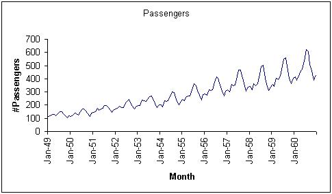
Example of a time series data set: Monthly airline bookings.
A time series model is first used to obtain an understanding of the underlying forces and structure that produced the data, and secondly, to fit a model that will predict future behavior. During analysis of the data, a model is created to uncover seasonal patterns or trends in the data (i.e., bathing suit sales in June). In the second step, forecasting, the model is used to predict the value of the data in the future (i.e., next year's bathing suit sales). Separate modeling methods are required to create each type of model.
Analytic Solver Data Science provides two techniques for exploring trends in a data set: ACF (Autocorrelation function), and PACF (Partial autocorrelation function). These techniques help to explore various patterns in the data that can be used in the creation of the model. After the data is analyzed, a model can be fit to the data using Analytic Solver Data Science's ARIMA method.
Autocorrelation (ACF)
Autocorrelation (ACF) is the correlation between neighboring observations in a time series. When determining if an autocorrelation exists, the original time series is compared to the lagged series. This lagged series is simply the original series moved one time period forward (xn vs xn+1). Suppose there are five time-based observations: 10, 20, 30, 40, and 50. When lag = 1, the original series is moved forward one time period. When lag = 2, the original series is moved forward two time periods.

The autocorrelation is computed according to the formula:

Where k = 0, 1 , 2, ... n; Yt is the Observed Value at time t; Ybar is the mean of the Observed Values and Yt –k is the value for Lag-k.
For example, using the values above, the autocorrelation for Lag-1 and Lag - 2 can be calculated as follows.
 = (10 + 20 + 30 + 40 + 50) / 5 = 30
r1 = ((20 - 30) * (10 - 30) + (30 - 30) * (20 - 30) + (40 - 30) * (30 - 30) + (50 - 30) * (40 - 30)) / ((10 - 30)2 + (20 - 30)2 + (30 - 30)2 + (40 - 30)2 + (50 - 30)2) = 0.4
r2 =( (30 - 30) * (10 - 30) + (40 - 30) * (20 - 30) + (50 - 30) * (30 - 30)) / (((10 - 30)2 + (20 - 30)2 + (30 - 30)2 + (40 - 30)2 + (50 - 30)2) = -0.1
The two red horizontal lines on the graph below delineate the Upper Confidence Level (UCL) and the Lower Confidence Level (LCL). If the data is random, then the plot should be within the UCL and LCL. If the plot exceeds either of these two levels, as seen in the plot above, it can be presumed that some correlation exists in the data.

Partial Autocorrelation Function (PACF)
This technique is used to compute and plot the partial autocorrelations between the original series and the lags. However, PACF eliminates all linear dependence in the time series beyond the specified lag.
ARIMA
An ARIMA (Autoregressive Integrated Moving Average Model) is a regression-type model that includes autocorrelation. The basic assumption in estimating the ARIMA coefficients is that the data is stationary -- the trend or seasonality cannot affect the variance. This is generally not true. To achieve the stationary data, Analytic Solver Data Science first applies differencing: ordinary, seasonal, or both.
After Analytic Solver Data Science fits the model, various results are available. The quality of the model can be evaluated by comparing the time plot of the actual values with the forecasted values. If both curves are close, then it can be assumed that the model is a good fit. The model should expose any trends and seasonality, if any exist. If the residuals are random then the model can be assumed a good fit. However, if the residuals exhibit a trend, then the model should be refined. Fitting an ARIMA model with parameters (0,1,1) will give the same results as exponential smoothing. Fitting an ARIMA model with parameters (0,2,2), will give the same results as double exponential smoothing.
Partitioning
To avoid over-fitting of the data, and to be able to evaluate the predictive performance of the model on new data, first partition the data into Training and Validation Sets using Analytic Solver Data Science's time series partitioning utility. After the data is partitioned, ACF, PACF, and ARIMA can be applied to the data set.
